Need help dealing with dates in SUMIFS formulas (after updating LO from 6.3 to 7.6.2)

This site changes straight quotes to curly quotes unless it is inside the ` for preformatted text.

I copied your SUMIFS, corrected the curly quotes and it didn’t work but LO suggested a change which looked identical and it worked so maybe there is a zero width space or something in there. Make sure Enable Wildcards in formulae is ticked in Tools > Options > LibreOffice Calc > Calculate

SumifsWithDate.ods (18.1 KB)

1 Like

https://ask.libreoffice.org/uploads/short-url/uMwhnNnlcKMK2vj9JcprE4i3NPb.ods

1 Like

Please attach a sample file that worked in 6.3.

@mariosv @mikekaganski
A new sample it’s not necessary because it’s basically like the one EarnestAI sent. He used my example formula and his SUMPRODUCT formula.

You’ll notice that if you change the Date Format to DD/MMM, his SUMPRODUCT formula keeps working and my SUMIFS formula breaks after recalculating (changes to zero).

So far, nobody gave me an option using SUMIFS while keeping a DD/MMM format, but it’s ok. I’m assuming it’s not possible.

So you know what I need to see your issue. Bye then.

In @Ernest sample, both function works for me. So without your sample, how can we know what is not working?
But let’s go, it’s you asking for a solution.

So, did you change the date Column format to DD/MMM and the SUMIFS formula kept working? Do a Recalculate to double-check.
Or maybe it’s really just in my LibreOffice (maybe some configuration).

If you change the formula criteria, to not have the first slash, it works in both formats, DD/MM/YYYY or MM/YYYY

=SUMIFS(O5:O105;T5:T105;"*03/2022";A5:A105;"C")

Maybe something to do with The COUNTIF and COUNTIFS functions mis-count on mixed numeric and text data and query by string

Likely not, because that was a failure of 7.4.0 fixed in 7.4.7.2 and 7.5.3.2 and 7.6.0, whereas the OP said upgrading from 6.3(.whatever) to 7.6.2.

The "*/03/2022" depends on the format of the date cell values, so changing that will make things fail. With DD/MMM format you’d have to use "*/Mar" instead, but obviously that lacks the year so filtering for 2022 is not possible. The SUMPRODUCT() approach is the format independent solution here. Using SUMIFS() you can do similar with

=SUMIFS(O5:O105;YEAR(T5:T105);2022;MONTH(T5:T105);3;A5:A105;"C")

entered as array formula (close with Ctrl+Enter instead of just Enter), but there’s no benefit in it over using SUMPRODUCT(), au contraire, it might be slightly slower.

1 Like

In defense of SUMIFS (not array formula): :slightly_smiling_face:

=SUMIFS(O5:O105; T5:T105; ">=" & DATE(2022;3;1);T5:T105; "<=" & DATE(2022;3;31);A5:A105;"C")
2 Likes

SUMIFS being significantly faster (and less stressful) than SUMPRODUCT is a myth? I’ve read about it somewhere.

I’m using a lot of SUMIFS+SUMIFS non-array formulas for my multiple conditions… I’m trying to learn how to use OR (and maybe AND) functions that maybe I can use to reduce my formulas in the future. Also, some people suggested pivot tables, I may take a look at this approach too.

Anyway, I’m already converting some of my formulas to value for the old data (values that will not be changed anymore). I think it will help to reduce stress in the file. Although, I’m not sensing any “lag” or anything while using this sheet, for now.

Thanks for your suggestion.

It depends… (read where?) on data and data layout (i.e. are there blank unused cells that don’t match the criteria anyway) and query. What SUMPRODUCT() does it creates interim arrays of all arguments and then just multiplies the positional values. With many blank or non-matching cells in a to-be-summed range like O5:O105 (but larger) creating an array is an unnecessary overhead. SUMIFS() uses query cell iterators for the conditions over ranges, creates a result array, and for fulfilled conditions asks cells in the to-be-summed range. With many fulfilled conditions that is slower, with less it is faster. On the other hand, creating an array of a cell range of contiguous numeric values (not formula cells) to be multiplied later by SUMPRODUCT() is faster if more cells match the condition than don’t. But those are implementation details. So yes, in general for large ranges SUMIFS() is probably faster and takes less memory, for small ranges it doesn’t matter, but formulating the conditions for SUMPRODUCT() may be more straight forward as all SUMIFS() conditions can only test for equality whereas the interim arrays of SUMPRODUCT() arguments may be results of any comparison.

1 Like

You could use the SUMPRODUCT function in this way:

=SUMPRODUCT(O5:O105;YEAR(T5:T105)=2022;MONTH(T5:T105)=3;A5:A105=“C”)

What this function does is for each row, it takes the values of each argument then it multiplies them together. It then makes the sum of all these values for all the rows.

The trick here is when the year is 2022, the equality is 1, when the month is 3 the equality is 1, but if the year is 2023 for example, the result is 0 and then the multiplication of all arguments for that row is 0, which adds 0 to the sum.

Of course, you will need to change all your formulas…

1 Like

Ok, your SUMPRODUCT formula is working with the DD/MMM date format (and @EarnestAl example sheet is working too).

Can I use a SUMIFS formula with these “YEAR” and “MONTH” as conditions? I tried, but it leads to error…

I don’t need them to “multiply” as you said… And I’ve read somewhere that SUMIFS calculates significantly faster than SUMPRODUCT, should I ignore that? (I’m talking about 200+ different SUMIFS formulas in a single sheet).

Should I avoid the SUMPRODUCT and just go with the “tricky” way I mentioned? (I mean add an extra hidden column with the date in other format, just for the formula sake).
Honestly, this would probably be faster than fixing all formulas, lol.

Thanks for the help already, guys!

Sounds like you should use a pivottable as @villeroy has already provided

It does even work with currency format or any other number format because a number format does not change any value.
97023.ods (16.1 KB) (same thing in all popluar spreadsheets of the past 3 decades)

1 Like

Both @EarnestAl and @Steph1 SUMPRODUCT formulas are very valid solutions. Thank you, guys!

But changing all my sumifs formulas in the sheet would be too much work. I’m also not 100% sure if all my other formulas conditions would be viable with a sumproduct formula…

So I decided to just add an extra column that copies my DD/MMM cells (where I’ll look and insert the data everyday) to a DD/MM/YYYY format column (That I’ll keep hidden, just for the formulas’ usage).

By doing that, I ran into a problem: My blank date cells were copying to a “30/12/1899” date in the new column, instead of a blank cell. But I already solved that problem by using the function:
=IF(T5="";"";T5)
This way, the blank T cells returns to blank cells in the new column, as intended.

Thanks, everyone, for the replies.

The pivot table solution as proposed by @Villeroy is the easiest and quickest solution and least likely to to require tweaking for exceptions.
SumifsWithDate&Pivot.ods (21.0 KB)

2 Likes

Damn, I have no idea how to create this.
But I’ll keep the sample to someday learn how to do it. Thanks!

Using the sample:

  1. Select cells A4:T105

  2. Click Data > Pivot Table > Insert or Edit. OK Current Selection

  3. In the dialogue, Pivot Table Layout, that opens, drag Date into Row Fields, Letter into Column Fields, Value into Data fields (it will automatically choose Sum). Click OK

  4. In the newly created pivot table on a new sheet, click in the Date column. Click Data > Group and Outline > Group.

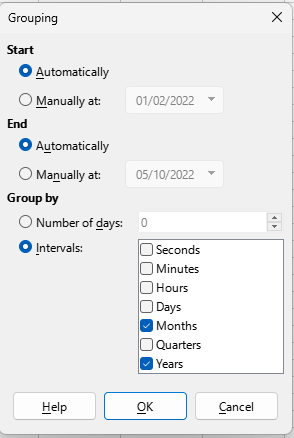
  5. In the new dialogue, Grouping, under Group by, make sure both Months and Years are ticked. This will separate months from different years. OK and done.
    GroupingYearMonth

If you want to move the pivot table, right click on it, select Properties. Expand Source and Destination, click the shrink button next to Destination Selection and click where you want the pivot table to be.

If there are other columns you want summed, then click Properties and drag into Filter or Column or Row depending on how you want to see your data. You can have more than one field in any pane.

To change from Sum Value, double-click on it to select, Count, Average, etc.

Play around with it to familiarise yourself with how it works. Cheers, Al

3 Likes