
Hello guys!
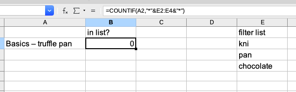
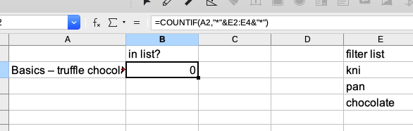
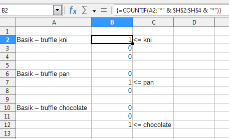
I try to find any of the text in the filter list (E2:E4) within cell A2. The formula I found is returning “1” only for the first word in the filter list, i.e. kni. 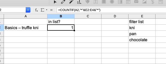
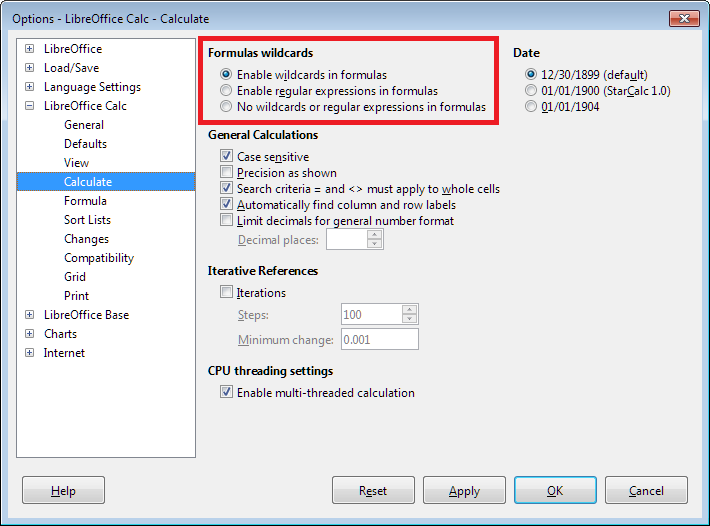
It does not work for “pan” or “chocolate”. Regular expressions are enabled.
I appreciate the help as always!
Sophia
FOLLOW UP QUESTION:
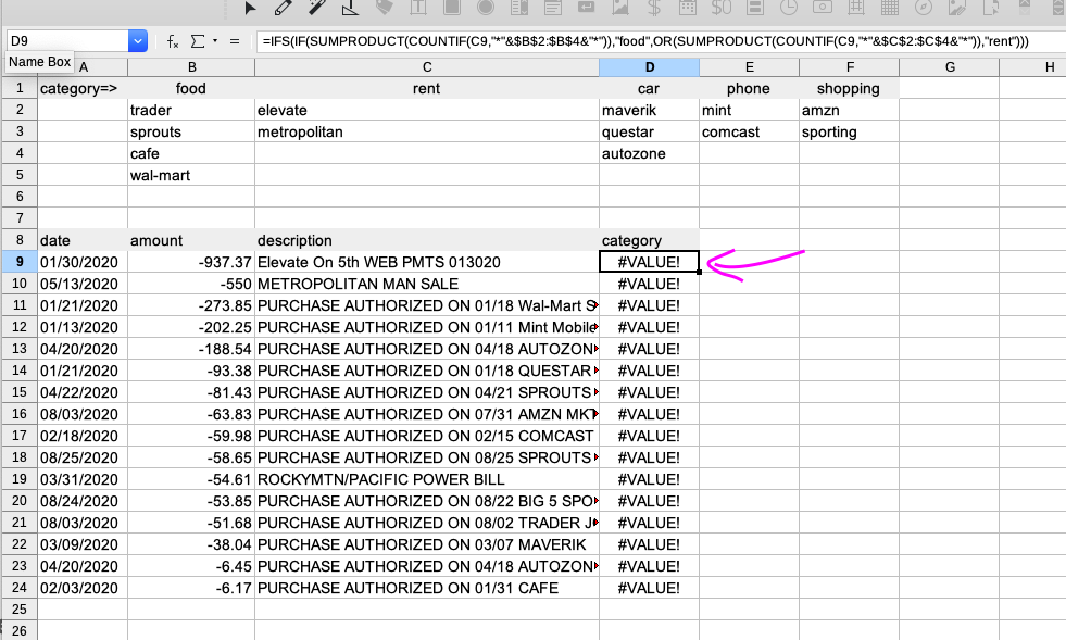
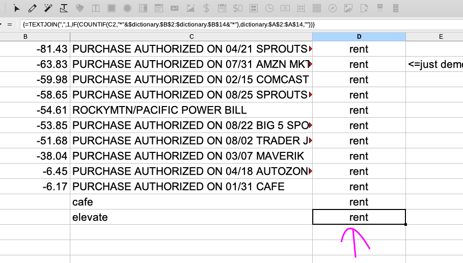
This is what I have in mind: an accounting sheet with categories assigned to transactions from my bank account.
Categories are Food, Rent, Car, Phone, Shopping, with filter words in each of the categories.
I want the formula to search C colume, starting at C9, and assign a catogory in D colume same row (pink arrow) based on the work of what filter list was found. E.g. if the description contains “cafe”, category “Food” is assigned. If the description contains “maverik”, category “Car” is assigned. Etc. Please see img and ODS file below:
Here is the actual ODS file: example.ods
EXAMPLE FILE 2: the array formula does not work after adding two new inputs (cafe, elevate) in the C colume.

 I go into editing my answer (or question), use the usual tools for inserting files or images, cut the resulting strings, click Cancel so as not to spoil the existing answer, and paste the copied rows into the comment. (for example, here I paste text