How to lookup a column with multiple exact match results and find a value in the next column higher or equal to a calculated formula?

[MaxKnight1010101]

So I’m working on a spreadsheet to chart out all of the possible fusion results in the first Persona game. I’ve already got the list of demon cards both horizontally and vertically, and I had started on filling in the resulting personas by hand, but came to realize that it would take far to long doing it that way.

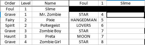
The tarot result of the fusion is what I want to match with, while the number that is there would be the resultant level based on the following formula:

=ROUNDDOWN(AVERAGE(E1,$B3),0)+3

I need to use the lookup to match one thing, the tarot that is in all capitals in column D there. From there, on the sheet I’m doing the lookup on, I need to use the calculated number in column E shown above to find the level number of the first persona that is greater than or equal to that calculated number, with equal to taking precedence.

The problem is twofold: one, there are multiple possible results of the exact match lookup; two how to join that lookup to find the value we want from the second sheet. There’s a further complication I can see occurring, though.

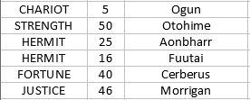
There are instances where there are only one possible result, meaning it doesn’t matter if the input we would get out of the previously mentioned formula is higher than the value we can lookup, it needs to match up with it anyways. I know for this one, I could do a simple VLOOKUP and get the exact match and just fill it in for those, but if I can, I would like to use the same formula for all of these to make copying it across the board simpler (141 rows by, uh… columns going to PJ).

I am hoping this community can provide some insight!

EDIT: I have attached below the relevant portion of the workbook I’m dealing with, including the suggested solution from Lupp. I’m not sure if it’s because I’m trying to inline the solution, or if OFFSET just doesn’t work when referencing a separate Sheet (Data to match up is on Sheet6, but the table I’m building is on Sheet3_2). Formula that I’m using is below the attachment link.

PersonaTest.xlsx

=OFFSET($Sheet6.$A$2,(MATCH(1,($Sheet6.$A$2:$A$58=D$3)*($Sheet6.$B$2:$B$58>=(ROUNDDOWN(AVERAGE(E$1,$B3),0)+3)),0))-1,0,1,2)

[mariosv]

Pls can you attach a sample file (edit your question to do it) with notes about what you want to achieve.

[Lupp]

Concerning the described task this should be a solution:
ask291784matchTwoConditions_1.ods
(Wouldn’t study that much image area.

[MaxKnight1010101]

I have edited the post to include the portion of my workbook that I’m dealing with, along with my attempt to implement Lupp’s solution. I’m getting #VALUE as a result of my attempt at it.

[Lupp]

Always simplify things.
This is mainly important while still functionality needs to be implemented. Special formatting, moving parts of the data elsewhere, and the like may be done if everything is working well already.
Always use the native “file formats” of LibreOffice (ODF-specified).
I still wouldn’t like to dive into your special use-case. That’s not my cup of tea. You are looking for help, I assume, not for a final solution.
As far as I understood the question based on the explanations, the attached document should help you to find a way to accomplish your thing.
gameThing1.ods
I didn’t understand the absolute row-addressing you used in the formula. The calculations used in the second comparison should be done in a helper column once for all the formulas needing them.

[MaxKnight1010101]

I’m afraid I can’t simplify this any more than it already was. Each set of three columns in the original sheet would need its own separate lookup column, as we need to take the average of the level from each row and column and add 3 to get the level that is used as part of the lookup (where we are checking the second sheet for either an exact match or if not found, the next highest match if at all possible). I was able to modify the OFFSET solution to find the numbers correctly from off of the separate sheet (changed the column and width numbers from 0 and 2 to 1 and 1), but it fails when the average +3 is higher than the possible level I’m looking up. I think I have a couple solutions in mind to fix that, though; I’ll add the answer once I’ve got it.

[Lupp]

First of all you need to explicitly enter formulas relying on array-evaluation in the correct way.
Additional columns (helpers) are much better than convoluted formulas.
Of course you may need to accept complications depending on the actual task. But obey an advice very often useful and surely with everything roughly being “programming”:
Analyse the problem top-down.
Having separated levels, you can start to implement efficient solutions bottom up.
Trying to do both steps in one may end with a bloody nose.
E.G.: Having created a few helper columns and finding it wouldn’t badly afflict efficienc to integrate the calculation ino a superordinate formula, you can easily do so. During development the split formulas are much more helpful.
Where extreme efficiency is required, the problem needs a very specific review.

[Lupp]

Using spreadsheets: You often develop with a small sample of data, and you hope (ore simply assume) your concepts will well scale to the later needed size.
Many solutions contain elements with a so-called time-complexity much worse than linear (often quadratic). What worked well for 50 rows may then still be theoretically correct, but unusable with 500 rows.

[MaxKnight1010101]

So as I said in my comment above, the OFFSET solution was indeed correct, but needed to be modified slightly to make it work.

OFFSET($Sheet6.$A$2,MATCH(1,($Sheet6.$A$2:$A$58=D3)*($Sheet6.$B$2:$B$58>=(ROUNDDOWN(AVERAGE(E$1,$B3),0)+3)),0)-1,1,1,1)

This worked up until the value from the AVERAGE + 3 was higher than any of the values in the table we were looking up on Sheet6. I came to realize that I would actually need a second table on Sheet6 that only included the highest entry for each value we would be looking up, and a logical IF to determine if we should use the first or second table:

=IF((ROUNDDOWN(AVERAGE(E$1,$B3),0)+3)>OFFSET($Sheet6.$E$2,MATCH(D3,$Sheet6.$E$2:$E$22,0)-1,1,1,1),OFFSET($Sheet6.$E$2,MATCH(D3,$Sheet6.$E$2:$E$22,0)-1,1,1,1),OFFSET($Sheet6.$A$2,MATCH(1,($Sheet6.$A$2:$A$58=D3)*($Sheet6.$B$2:$B$58>=(ROUNDDOWN(AVERAGE(E$1,$B3),0)+3)),0)-1,1,1,1))

I junctioned this solution to also auto fill in the names that would be associated with the level I looked up with the previous formula, repeating it in the next column but changing the Column offset from 1 to 2. A quick copy-paste-paste filled in the formula for the rest of Sheet3_2 and using Find/Replace to clean up all of the #N/A from the table and conditional formatting to give the blank cells a black background… I now have a completed table far faster than if I’d looked up and filled this in by hand.

Thank you, Lupp, for pointing me in the right direction; I’d never used OFFSET or MATCH before so this was an education. The completed, filled-in workbook: PersonaTestComplete.xlsx