
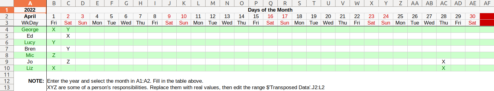
I wonder how to create a summary table based on categorical data. In the attached file, sheet#1 is the time table for my company; column#1contains the employees names, column#2-31 are the days of the month. X, Y and Z are the type of duty they are assigned to that specific date. How can I automatically create a summary table like the one on Sheet#2 where the dates are the rows whereas the columns are the X, Y, and Z (the duties).
Example 1.ods (9.8 KB)
The table in your example_1.ods is not a normalized table. With a normalized table you have plenty of options at hand.
Pivot_Mont_Person_Category.ods (67.1 KB)
has a normalized table in columns A through D.
One row of column labels. Actual data rows below this label row.
One column of dates.
One column of category names.
One column of person names.
One column of decimals.
The header row has auto-filter buttons.
The table can be sorted by any of the 4 columns without spoiling the information.
Dozends of formula functions presume normalized tables.
A pivot table is a cross table (aka contingency table) generated from a normalized table without a single formula.
2 Likes
Welcome!
The formula may seem complicated:
{=TEXTJOIN(". ";1;IF(OFFSET(Sheet1.$A$2:$A$8;0;MATCH($A2;Sheet1.$B$1:$Y$1;0))=B$1;Sheet1.$A$2:$A$8;""))}
In fact, everything is quite simple.
MATCH($A2;Sheet1.$B$1:$Y$1;0))=B$1 found the number of the column with the date from the current row from column A
OFFSET(Sheet1.$A$2:$A$8;0;<column number>) finds all values from the desired column
IF(<array value>=B$1;Sheet1.$A$2:$A$8;"") Compares the values of the column cells with the heading of the current column and, if the values match, substitutes the name, otherwise an empty string
And finally, TEXTJOIN() concatenates the found values into one line through the delimiter.
Since inside the formula the whole range is compared with one value, then this is an array formula, the input should be completed with the key combination Ctrl+Shift+Enter (the curly braces around the formula mean exactly that - the array formula)
Here’s what it might look like with your sample data - Example 1.ods (21.4 KB)
2 Likes
It is not so easy when the first argument of the OFFSET function is a range.
Try this.
transposed-data.ods (29.4 KB)
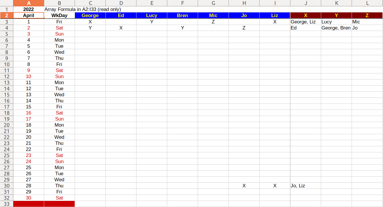
X: {=TEXTJOIN(", ";1;IF($C4:$I4=J$3;$C$3:$I$3;""))}
Edit 1:
File updated
Conditional Formatting:
B2:AF3: Formula is OR(B$3=TEXT(WEEKDAY(0);"NN");B$3=TEXT(WEEKDAY(1);"NN")) to meet Sat (Saturday) & Sun (Sunday), colored red.
Edit 2:
The attached file has been updated (complete data). The $Transposed Data’.C:AO columns can be hidden.
transposed-data (2).ods (44.1 KB)
1 Like
Updated. Minor bug fixes.
Thanks very much, grateful for your sincere help.
I tried adding more employees and types of duties, edited the formula. however, it always returned ERR508.
I am using libreoffice 7.3 on Debian linux
attached an example
Example 2.ods (21.2 KB)
The attached file in the solution has been updated (complete data). See ‘transposed-data (2).ods’. The $Transposed Data’.C:AO columns can be hidden.
In the range $‘Transposed Data’.AP3:AU33, copy any one cell with the formula and paste it into any number of pre-selected other cells in the specified range. This is an array formula. Dragging it with the mouse does not work. The formula does not need to be drawn up manually.
1 Like
X: {=TEXTJOIN(", “;1;IF($B2:$AN2=AO$1;$B$1:$AN$1;”"))}
First, I replaced the delimiter (but that may not be the point), and second, I have the number of array formulas equal to the number of cells (one cell - one formula), while you have one general array formula for all cells. Feel the difference!
But the array formula for transposing a range is the only one.
1 Like
Thank you very much, I think the issue has been solved. I think I,kind of, understood the formula now.